
Top ten ways to clean your data in excel
In his day and age, our dependence on data is overwhelming. Thanks to our cellphones and laptop, a halo of data surrounds our life. Data is nothing but a piece of classified information.
Microsoft Excel is one of the most used data handling/analysis software. At the same time, one tiny mistake in analyzing data can cause headaches. Simple errors like spacing, value error, format, duplicates, etc. usually miss our eye.
Imagine the chaos when you handle large chunks of information. Keeping your Data clean and organized can take you miles ahead in your work ethics and efficiency.

Here’s a list of Top 10 Super Neat Ways to Clean Data in Excel as follows.
1) Get Rid of Extra Spaces:
Extra Spaces are difficult to spot & correct. Multiple spaces may be easy, but trailing spaces are pretty tough. Trailing spaces are blank spaces at the end of the statement or word which are not followed by any other character.
Here’s an easy way to spot & eliminate such errors:
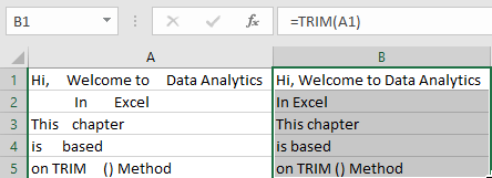
Syntax: TRIM(text)
Steps:
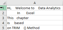
- Consider data with four cells with different spacing errors.
- Now select a column & type “TRIM(“
- Now select the cell you want to correct (in matters of spaces).
- The cell will be corrected. If there are other erroneous cells sequentially aligned, drag the fixed cell till the point, you want to check & correct.
This easy step can save you time!
2) Select & Treat all blank cells:
Blank cells are troublesome because they often create errors while creating reports. And, people usually want to replace such cells with 0, Not Available or something like that. But replacing each cell manually on a large data table would take hours. Luckily, there’s an easy way to tackle this problem.
Steps:
- Select the entire Data (you want to treat)
- Press F5 (on keyboard)
- A dialogue box will appear > Select “Special”
- Select “Blanks” & click “OK”
- Now, all blank cells will be highlighted in pale grey color, out of which one cell would be white with a different border. That’s the active cell, type the statement you want to replace in blank cells.
- Hit “Ctrl+Enter”
NOTE:
At the last step, if “Enter” only is pressed, then the value will be inserted only in the active cell. So remember to press “Ctrl+Enter.”
3) Convert Numbers Stored as Text into Numbers:
When we import data from files, other sources, databases, text, etc. During transit, data might get affected. Also, some have a habit of using an apostrophe before numerical values, which is considered as text in Excel. Such minor data conversion can drastically affect calculations.
Suppose there are three values “70, ’70, 80”. When we compare 70 and 80 (70<80), the result is “TRUE.” But when we compare “apostrophe 70 & 80” (‘70<80), the problem starts. Here the result will be FALSE as the text will be rated higher than any number. To eliminate such errors, here’s a trick.
Steps:
- Select any blank cell & type 1
- Select that cell & hit “Ctrl+C”
- Now select your data set & go to Paste > Paste Special
- In Paste Special, select “Multiply” option in the “Operation” category
- Click “OK”
Here it multiples every single value to “1”. And anything multiplied by 1 is the same number. But this trick also takes care of the apostrophe numerical.
4) Remove Duplicates:
Elimination of duplicate data is necessary for the creation of unique data & less usage of storage. In duplication, you can either highlight it or delete it.
A) Highlight Duplicates:
- Select the data & go to Home > Conditional Formatting > Highlight Cell Rules > Duplicate Values
- A dialogue box will appear (Duplicate Values), Select Duplicate & formatting color
- Press OK
- All duplicate values will be highlighted!
B) Delete Duplicates:
- Select the data & go to DATA > Remove Duplicates
- A dialogue box will appear (Remove Duplicates), tick columns whose duplicates need to be found.
- Remember to have a click on “My data has headers” (if your Data has headers) or else column heads will be considered as data & duplication search will be applied on it too.
- Click OK!
Duplicate values will be removed! Suppose you select 4 of 4 columns. Then that four columns rows should also match or else; they won’t be considered duplicate.
5) Highlight Errors:
While creating reports or dashboards, you might face a few arithmetical errors (like divisional errors). Such errors are easy to spot if the Data is small. But for big data, it’s complicated. So to get rid of such mistakes, you can go for two ways: Conditional Formatting or Go to Special.
A) Using Conditional Formatting:
- Select the Data
- Go to Home > Conditional Formatting > New Rule
- Within New Rule, Select “Format only cells that contain.”
- In Rules, Select “Errors” & Click on “Format”
- Select any color & click OK
- Hit the final “OK” button
All the cells with errors are highlighted & now are easy to spot.
B) Go to Special:
- Select the Data
- Press F5
- Click on “Special”
- A dialogue box appears (Go to Special), Select Formulas
- Now you get four options in Formulas, deselect all options except “Errors”
- Click OK! Now all errors are selected, you can delete them manually or replace a statement.
- If you wish to replace, then type the statement at active cell & hit “CTRL+ENTER.”
6) Change Text to Lower/Upper/Proper Case:
While importing data, we often find names in irregular forms like a lower, upper case, or sometimes mixed. Such errors are not easy to eliminate manually. Here’s a fingertip trick to bring back the consistency.
- LOWER(text)
- UPPER(text)
- PROPER(text)
Steps:
- Just type the formula you want to use, suppose “LOWER(“ and select the cell whose case needs to be changed.
- Hit “CTRL+ENTER.”
- The case has been changed & consistent
- Drag down to do the same for other cells.
- Similarly for UPPER() & PROPER()
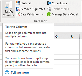
7) Parse Data Using Text to Column:
Sometimes the received Data has texts filled in one cell, only separated by punctuations. Usually, the addresses are cramped in one cell separated by a comma. To distinguish values in separate cells, we can use “Text to Column.”
Steps:
- Select the Data
- Go to Data> Text to Column
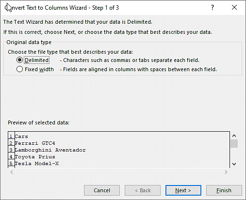
- A dialogue box will appear (Convert Text to Columns Wizard – Step 1 of 3), select Delimited or Fixed Width as per your convenience.
- Delimited is to be selected if the width isn’t fixed, click “NEXT”
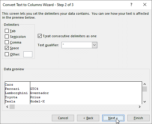
- In Delimiters tick the option which separates your text in the cell. Suppose “Norwich Cathedral, Norwich, UK,” here three values are separated by commas. So we will select “Comma” for this example. And, deselect rest options.
- View the preview & click on “NEXT”
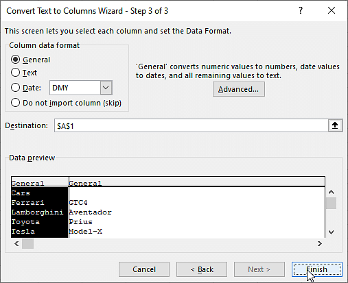
- Select Column Data Format & destination cell address
- Click “FINISH”
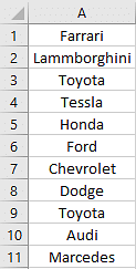
8) Spell Check:
Spelling mistakes are common in text files & PowerPoint. However, MS points out such errors by underlining it with colorful dashes. And, MS Excel doesn’t have such feature. But you can use it below steps:
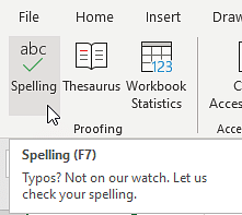
- Select the Data
- Press “F7”
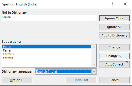
- A dialogue box appears, which shows you the possible wrong word & it’s the possible correct spelling. Click on “Change,” if you agree with the suggestion.
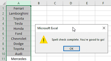
- Check & change till it says “Spell check complete. You’re good to go!”
9) Delete all Formatting:
Suppose you want to clear all the formats, including highlights & borders. You can do this by selecting the data & go to HOME > Clear (in editing group) > Clear Formats. It will clear the formats & you get standard content without highlights or borders. Similarly, you can clear Content, Comments, Hyperlink, or entire data (using Clear All).
10) Use Find & Replace to Clean Data in Excel
A) Changing Cell References:
- Press “CTRL+H” to open “Find and Replace”
- Now in Replace > “Find What” (change the reference range too) “Replace With”
- Suppose Find What: $B to Replace With: $C
- Click on “Replace All”
- Similarly finding & replacing using reference range we can clean the Data
B) Find & Change Specific Format:
- Press “CTRL+H”
- Select “Options”
- Now go to “Format” of “Find What.” Here you can specify the format or choose a format from the cell. Suppose you select a format.
- Now it will show you the preview for “Find What.”
- Click on “Format” of “Replace With.” Suppose we go for “Format…”
- Now select format, example: Number, Alignment, Font, Border, Fill, Protection.
- Suppose we select Color then select any color to fill the column header cell.
- Click on Replace All
- Instantly the format has been changed!
C) Removal of Line Breaks:
Suppose we have a data where it is separated by line breaks (same cell but different rows). To remove these line breaks, follow the below steps:
- Press “CTRL+H”
- Find and Replace dialogue box will appear, press “CTRL+J”
- Go to the replace with box & type a single space
- Click Replace All
- All rows will be managed in one row within the same cell!
D) Removal of Parenthesis:
- Select the Data
- Press “CTRL+H”
- Type (*) in “Find What” (This will consider all characters within parenthesis)
- Leave the Replace With column empty & click Replace
- Parenthesis characters are removed!
Conclusion:
These were TOP 10 Super Neat Ways to clean data in Excel. We have discussed the elimination of different types of data errors in simple ways. I hope you liked it!

Some simple steps can easily do the procedure of Data Cleaning in Excel by using Excel Power Query. This tutorial will help you learn about some of the fundamental and straightforward practices for cleaning data in excel.
Make Data-Driven Business Decisions
Purdue PCP in Business AnalysisEXPLORE COURSE
How to Clean Data in Excel?
Remove Duplicates
One of the easiest ways of cleaning data in Excel is to remove duplicates. There is a considerable probability that it might unintentionally duplicate the data without the user’s knowledge. In such scenarios, you can eliminate duplicate values.
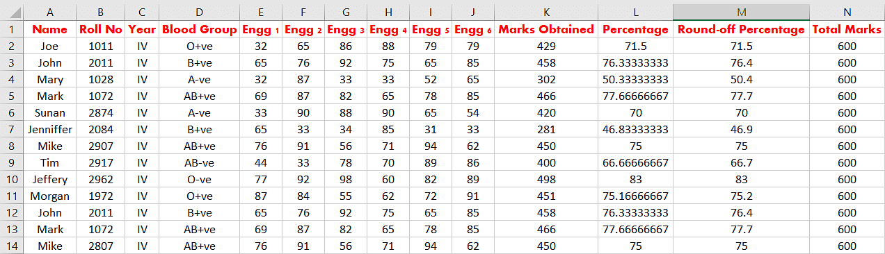
Here, you will consider a simple student dataset that has duplicate values. You will use Excel’s built-in function to remove duplicates, as shown below.
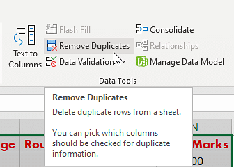
The original dataset has two rows as duplicates. To eliminate the duplicate data, you need to select the data option in the toolbar, and in the Data Tools ribbon, select the “Remove Duplicates” option. This will provide you with the new dialogue box, as shown below.
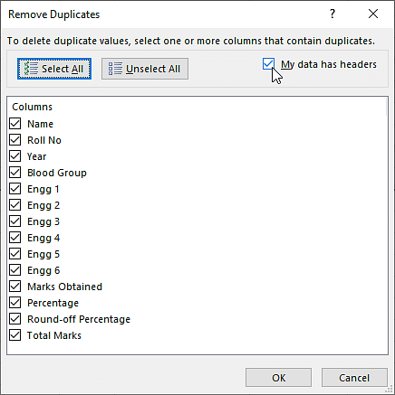
Here, you need to select the columns you want to compare for duplication. Another critical step is to check in the headers’ option as you included the column names in the data set. Excel will automatically scan it by default.
Next, you must compare all columns, so go ahead and check all the columns as shown below.
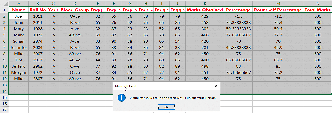
Select Ok, and Excel performs the operations required and provides you with the data set after filtering out the duplicate data, as shown below.
In the next part of Excel Data Cleaning, you will understand data parsing from text to column.
Data Science Career Boot Camp
The Ultimate Ticket to Top Data Science Job RolesEXPLORE COURSE
Data Parsing from Text to Column
Sometimes, there is a possibility that one cell might have multiple data elements separated by a data delimiter like a comma. For example, consider that there is one column that stores address information.
The address column stores the street, district, state, and nation. Commas separate all the data elements. You must now divide the street, district, state, and nation from the address columns into separate columns.
Excel’s inbuilt functionality called “text to column” can achieve this. Now, try an example for the same.
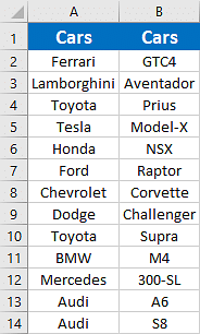
Here, you have the car manufacturer and the car model name separated by space as the data delimiter. The tabular data is shown below.

Select the data, click on the data option in the toolbar and then select “Text to Column”, as shown below.
A new window will pop up on the screen, as shown below. Select the delimiter option and click on “next”. In the next window, you will see another dialogue box.
In the new page dialogue box, you will see an option to select the type of delimiter your data has. In this case, you need to select the “space” as a delimiter, as shown below.
In the last dialogue box, select the column data format as “General”, and the next step should be to click on the finish, as shown in the following image.
The final resultant data will be available, as shown below.
Followed by Data parsing, in this tutorial about Excel Data Cleaning, you will learn how to delete all formatting.
UMN Business Analytics Bootcamp
Advance Your Business With Our Analytics BootcampENROLL NOW
Delete All Formatting
Another good way of cleaning data in excel is to ensure even formatting or, in some cases, even removing the formatting. The formatting can be as simple as coloring your cells and aligning the text in the cells. It can be a logical condition applied to your cells using Excel’s conditional formatting option from the home tab.
However, in situations where you wish to remove the formatting, you can do it in the following ways. First, try to eliminate the regular formatting. In the previous example, you took the case of car manufacturers and car models data tables with heading cells colored in blue, and the text was center aligned.

Now, use the clear option to remove the formats. Select the tabular data as shown below. Select the “home” option and go to the “editing” group in the ribbon. The “clear” option is available in the group, as shown below.
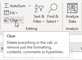
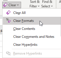
Select the “clear” option and click on the “clear formats” option. This will clear all the formats applied on the table.
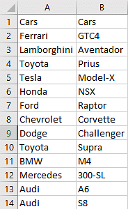
The final data table will appear as shown below.
Now, you must learn how to eliminate conditional formatting for cleaning data in Excel. This time, consider a different sheet. You must use the student’s details sheet, which includes conditional formatting in Excel.
To eliminate conditional formatting in Excel, select the column or table with conditional formatting as shown below.
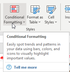
Then navigate to “Home”, and select conditional formatting.
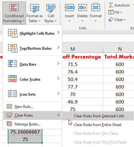
Then in the dialogue box, select the clear rules option. Here, you can either choose to eliminate rules only in the selected cells or eliminate rules from the entire column.
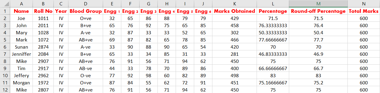
After you eliminate all conditions, the resultant table would look as follows.
You can always use a shortcut method to eliminate the conditional formatting in Excel. It is by pressing the sequential combination of the following keys as follows.
ATL + E + A + F
Next, in this Excel Data Cleaning tutorial, you will learn about Spell Check.
Business Analyst Master’s Program
Gain expertise in Business analytics toolsEXPLORE PROGRAM
Spell Check
The feature of checking the spelling is available in MS Excel as well. To check the spellings of the words used in the spreadsheet, you can use the following method. Select the data cell, column, or sheet where you want to perform the spell check.
Now, go to the review option as shown below.
Microsoft Excel will automatically show the correct spelling in the dialogue box, as shown below. You can replace the words as per the requirement as shown below.
The final reviewed data table will like the one below.
In the next segment of this Excel Data Cleaning tutorial, you will learn about changing the text case.
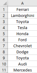
Change Case – Lower/Upper/Proper
You can manipulate the data in the Excel worksheet in terms of character cases as per the requirements. To apply case changes, you can follow the following steps.
Select the table or columns that need the case to be changed, as shown below.
Select the cell next to the column and apply the formula as per the requirement, as shown below.
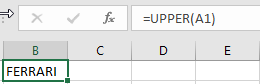
=UPPER(cell address) – for Upper case conversion
=LOWER(cell address) – for Lower case conversion
=PROPER(cell address) – for Sentence case conversion
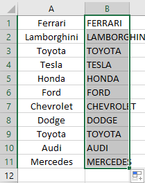
Now, you can drag the cell can to the last row, as shown below.
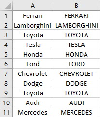
The final data table will appear as shown below.
Now that you learned spell check, in the upcoming section of Excel Data Cleaning, you will learn how to Highlight Errors in an Excel spreadsheet.
FREE Business Analytics With Excel Course
Start your Business Analytics Learning for FREESTART LEARNING
Highlight Errors
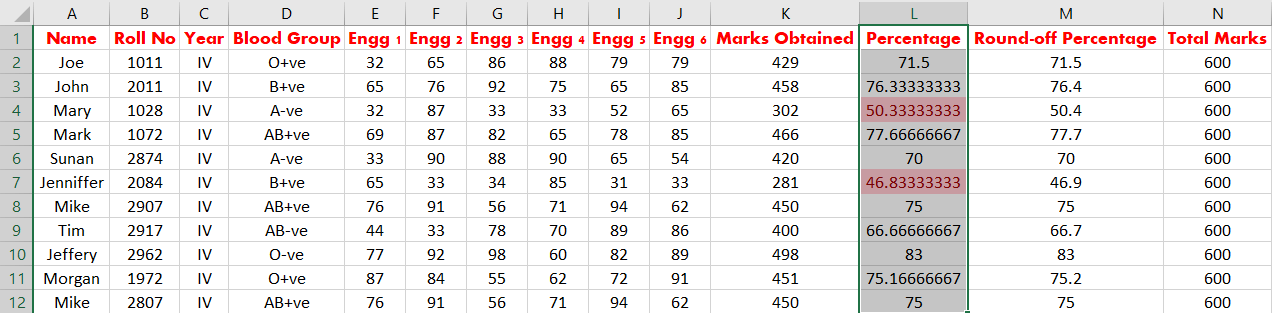
Highlighting errors in an Excel spreadsheet is helpful to find or sort out the erroneous data with ease. You can do error Highlighting with the help of conditional formatting in Excel. Here, you must consider the student data set as an example.
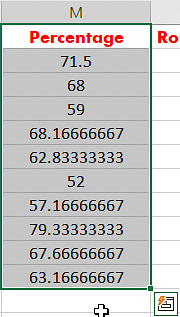
Imagine that you are interviewing all the students. There are eligibility criteria. You can shortlist the students if they have 60% aggregate marks. Now, apply conditional formatting and sort out the students who are eligible and not eligible.
First, select the aggregate/percentage column as shown below.
Select “Home”, and in the Styles group, select conditional formatting, as shown below.
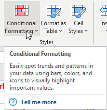
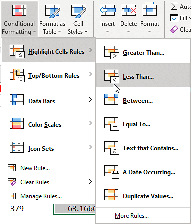
In the conditional formatting option, select the highlight option, and in the next drop-down, select the less than an option as shown below.
In the settings window, you will find a slot to provide the aggregate as “60” percent and press ok.
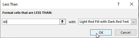
Excel will now select and highlight cells with an aggregate of less than 60 percent. In the next part of Excel Data Cleaning, you will understand the trim function.
TRIM Function
The TRIM function is used to eliminate excess spaces and tab spaces in the Excel worksheet cells. The excessive blank spaces and tab spaces make the data hard to understand. Using the “TRIM” function can eliminate these excessive blank spaces.
Select the data cells with excessive blank spaces and tab spaces. Now, select a new cell adjacent to the first cell.
Apply the TRIM() function and drag the cell as shown below.
It shows the final data after the elimination of the excess space as follows.
Next, in the Excel Data Cleaning tutorial, you will look at the Find and Replace function.
Find and Replace
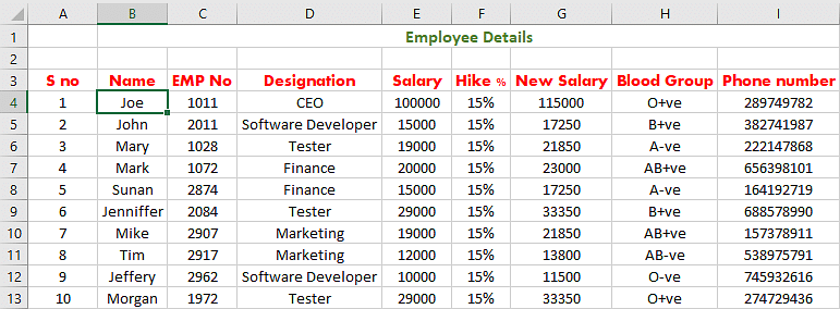
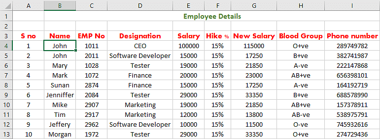
Find and Replace will help you fetch and replace data in the entire worksheet to help in organizing and cleaning data in Excel. Consider the employee data example.
Here, try to fetch an employee with the name Joe and try to rename or replace his name with John, after changing his first name.
The “find and replace” option is present in the home ribbon in the editing group, as shown below.
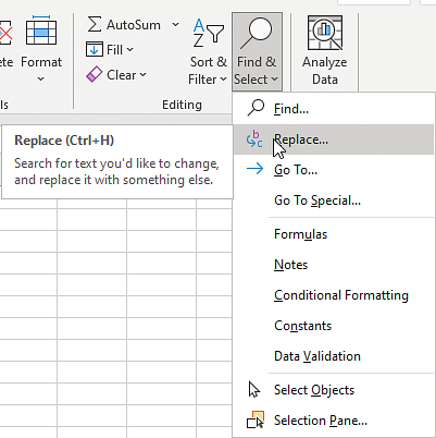
Click on the option, and a new window will open, where you can enter the data to be fetched and enter the text you need to replace, as shown below.
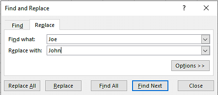
Click on “replace all”, and it will replace the text. The final dataset will be as shown below.
With that, you have come to an end of the “Excel Data Cleaning” tutoria
In this video, we answer “Why is Data Cleaning important?” and explore 10 incredibly useful Data Cleaning tips and tricks in Microsoft Excel to easily: ✅ Import a CSV using Text To Columns / Text Import Wizard ✅ Escape Commas in a CSV using Double Quotes ✅ Resize Columns using AutoFit ✅ Delete Blank Rows using Go To Special, Blanks ✅ Remove Duplicates ✅ Remove Excess Spaces in Text using the TRIM function ✅ Replace Values using Find and Replace ✅ Replace Formulas with Values using Paste Special, Values ✅ Standardise Text using UPPER, PROPER, and LOWER functions, and ✅ Standardise Dates
https://www.youtube.com/watch?v=H0tRB7M4VI8

Author: Editor
Views: 3
Leave a Reply