Users who have the subscription version of Excel receive regular updates that include new features and functions. An organisation’s update policy may affect the frequency of updates for business users.

Many of Excel’s new functions have been covered in detail in recent Excel Tips articles. Links have been provided.

1. Dynamic arrays

Dynamic arrays are a new way of calculating formulas and they are one part of Excel’s upgrade.

This new formula calculation method allows users to work with a range of cells the same way they used to work with an individual cell. This means a single formula can be created to populate a range. This range is called a spill range.

The formula appears in the top-left cell of the spill range. It can spill down, to the right or in both directions, creating a two-dimensional spill range. To refer to a spill range, add the # symbol to  the end of the top-left cell reference like A1#.

Dynamic arrays have been discussed in three previous articles that provide an overview, discuss the unique function and the filter function, and explain how to use them to sort lists.

2. XLOOKUP function

The XLOOKUP function replaces the VLOOKUP and HLOOKUP functions. To some extent, it also replaces the INDEX MATCH combination, which has been used in the past as a more flexible lookup option. XLOOKUP is now the preferred lookup function.

Click here for my comprehensive article on the XLOOKUP function.

3. LET function

The LET function allows users to create variables in formulas. This can shorten long and complex formulas and make them more efficient.

The LET function also works well with the new LAMBDA function discussed below.

Click here for my comprehensive article on the LET function.

4. TEXT functions

There are three new text functions that simplify extracting and manipulating text.

Click here for my comprehensive article on these three new functions.

5. LAMBDA function

The LAMBDA function allows users to create custom functions within Excel without VBA macros. Recently, other functions have been added so the LAMBDA function can include optional arguments when building custom functions.

The LAMBDA function is also required by some other new functions as part of their functionality.

Click here for my comprehensive article on the LAMBDA function.

6. ISOMITTED function

The ISOMITTED function works with the LAMBDA function. It identifies if optional custom function arguments have been omitted.

This allows users to set up default values for optional arguments, just like Excel’s built-in functions.

7. BYROW/BYCOL functions

There was an issue with dynamic arrays that can spill across and down when they were first released. It was difficult to refer to the rows and columns of a two-dimension spill range.

The BYROW and BYCOL functions have fixed that problem. They both require the LAMBDA function.

This article shows how to use both functions.

8. IMAGE function

The new IMAGE function enables a formula to display an image by extracting an image from a web address. The function requires an address with the HTTPS prefix to be used, so users cannot use images off personal hard drives or local servers.

Organisations could upload product images to their website. Business users could then use the IMAGE function to display those images based on a part number.

The companion video for this article demonstrates this function, with images that I have put on my own website.

9. VSTACK/HSTACK functions

The VSTACK and HSTACK functions provide many solutions to common issues that occur when trying to manipulate data and build reports.

The VSTACK function combines rows – V meaning vertical. This is like appending data where one table is added to the bottom of another table – see Figure 1 for an example.

The two separate lists of states in columns A and B have been combined into a single list, using a VSTACK function in cell D1. The VSTACK function creates a vertical spill range.

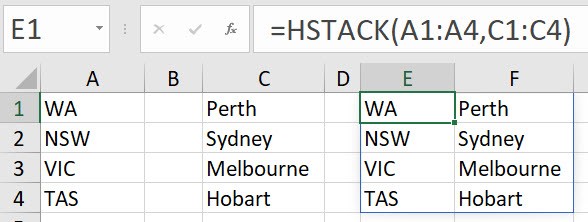
The HSTACK function combines columns of data and creates a multi-column table. The H stands for horizontal. In Figure 2, the list of states is in column A and the list of their respective capital cities is shown in column C. The HSTACK function in cell E1 combines the two separate lists into a two-column table.

The HSTACK function creates a two-dimensional spill range.

10. TAKE and DROP functions

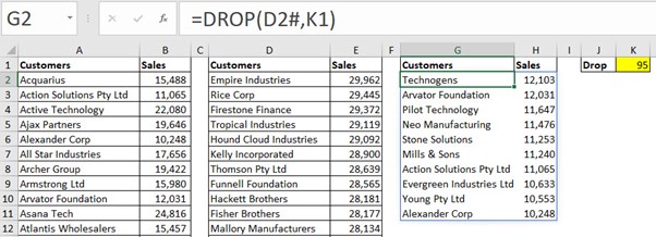
The TAKE and DROP functions allow you to extract entries from spill ranges. The TAKE function extracts either the first or last number of entries. In Figure 3, sales are listed by customer in alphabetic order in columns A and B. A SORT function in cell D2 creates a spill range that lists all the customers in descending order, based on their sales value.

We want to return a few of the top sales customers based on the value entered in the yellow cell K1. The TAKE function in cell G2 returns the first five rows from the sorted spill range. Note D2# refers to the spill range generated by the SORT function in cell D2.

If a positive number is used in the second argument of the TAKE function, it returns the first entries. If a negative number is used, it returns the last entries. See Figure 4, where -4 has been entered in cell K1. This returns the last four rows from the sorted spill range.

The DROP function specifies how many entries to remove. The customer list from the previous example had 105 customers. In Figure 5, the DROP function in cell G2 removes 95 of the customers from the top, leaving the bottom 10.

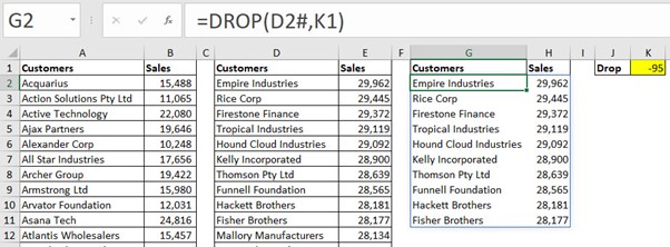
In Figure 6, using -95 in cell K1 removes the bottom 95, leaving just the top 10 sales.

Both TAKE and DROP can work with columns as they do with rows.

11. CHOOSEROWS and CHOOSECOLS functions

Dynamic arrays can create a two-dimensional spill range. You may then need to extract certain rows or columns from that spill range. The CHOOSEROWS and CHOOSECOLS functions simplify that process.

In Figure 7, cell B2 is generating a two-dimensional spill range summarising sales data by product and month from a data table in a separate sheet. Cell A7 has a dropdown that allows the user to select a product to plot on the chart.

The CHOOSEROWS function in cell B7 extracts from the spill range B2#. A number is used in the second argument of CHOOSEROWS to specify the row number to extract from the spill range. The MATCH function provides that number based on the product selected in cell A7.

CHOOSEROWS can extract more than one row, which is demonstrated in the companion video to this article. The CHOOSECOLS function works similarly, but it extracts columns from a spill range.

12. Other new functions

There are other new functions that have more complex uses, which also relate to dynamic arrays. These are:

• TOROW/TOCOL
• WRAPROWS/WRAPCOLS
• MAP
• REDUCE
• SCAN
• MAKEARRAY

13. New DAX functions

Excel’s PowerPivot feature allows Excel’s data model to be used to create reports based on relational databases. As part of that functionality, DAX functions can be used to create measures and calculated columns.

DAX functions are similar to Excel’s cell-based functions, but they are more powerful and flexible than Excel functions. They are also harder to master.

Excel’s PowerPivot DAX functions have remained the same for many years. That changed at the end of 2022 when 92 new DAX functions were launched.

These DAX functions are the same as the DAX functions available in Power BI.

Note that Power BI is updated more frequently and has more DAX functions than Excel. Knowledge from using DAX functions in Excel can be directly applied to Power BI.

Click here for my introductory article that explains and demonstrates basic DAX functions.